Lab 7: Modeling Friction Forces

Title:
Modeling Friction Forces

Purpose:
This lab's goal is to produce a model for friction based on measurements of mass and acceleration of an object moving on a uniform surface.

Theory:
The force of friction on an object is proportional to the normal force from the surface and a constant of either static or kinetic friction. Static friction of an object ranges from 0 to a maximum value where the object will remain at rest unless the applied force exceeds maximum static friction. The coefficient for static friction may be found if the mass of an object is known and the maximum force applied before the object moves is known. The coefficient for kinetic friction may be found if the mass of the object is known and the net force in the direction of motion is known. This is because kinetic friction remains a constant value as long as the object moves along the same surface. By making measurements to determine the maximum force of static friction and the acceleration of an object down a ramp of known incline, it is possible to find both constants and produce models predicting the behavior of an object with friction.

Apparatus:

• Block with linoleum tile surface (1)
• String
• Pulley (1)
• 5g hanging mass (1)
• Movable tabletop or board with flat plastic surface (1)
• Large quantity of 5g, 10g, 20g, and 50g masses
• 200g mass (3)
• Force sensor (1)
• Motion detector (1)
• LabPro (1)
• Computing device with Logger Pro software
• Angle measurement device (1)

Procedure:

Set the block on the flat plastic surface. Attach the hanging mass to the block using the string and place on the pulley. Slowly add mass to the hanging mass in 5g increments until the block begins to move. Subtract 5g from the total mass on the hanging mass and record as maximum static friction. Repeat these steps with 1, 2, and 3 added 200g masses on the block. Calibrate the force sensor and record the force as the block is dragged horizontally at a constant velocity across the plastic surface. Repeat this step with 1, 2, and 3 added 200g masses on the block. Place the block flat on the surface and slowly increase the incline of the surface and record the angle when the block begins to move. Attach a motion detector to the stop of the slanted surface and release the block again, recording its acceleration. Using calculated values of the coefficient of kinetic friction, predict the motion of the block as it is accelerated by a known mass. Use a motion sensor to measure the actual acceleration of the block.

Data and Graphs:

Photo of apparatus used in the experiment - Part 1

Photo of apparatus used in the experiment - Part 3

Velocity v time graph - Part 4

Velocity v time graph - Part 5

Calculations for uncertainties

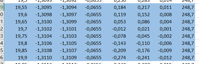
Table of data

Part 1	Mblock (g±0.1)	Mhanging (g±5)	μs	±
	187	100	0,535	0,0264639
	387	255	0,659	0,01275128
	587	350	0,596	0,00841275
	787	410	0,521	0,00628746
		Average μs	0,578	0,05488515
Part 2	Mblock (g±0.1)	Avg Force (N±0.001)	μk	±
	187	0,492	0,268	0,0004014
	387	1,045	0,275	0,0001921
	587	1,638	0,284	0,000125
	787	2,204	0,285	9,3097E-05
		Average μk	0,278	0,00082374
Part 3	Angle (°±0.1)	μs	±
	29,8	0,573	0,001922819
Part 4	Accel (m/s^2)	μk	±
	1,818	0,359	0,00019747
Part 5	Mblock (g±0.1)	Mhanging (g±0.1)	Calc. accel (m/s^2)	±
	187	105	1,272175582	4,1553E-05
		Actual accel (m/s^2)	1,346

Equations used (circled)

Analysis:

Using Newton's equation F=ma and the equations of friction, a value for the coefficient of static or kinetic friction was found in parts 1-4 of the experiment. Uncertainties were calculated for each coefficient of friction. Other equations used are shown in photos.

ww

Conclusion:

Our predicted acceleration in part 5 using the coefficient of kinetic friction found in part 4 was 1.272+-0.0000416m/s^2 and our measured acceleration was 1.346 m/s^2. Based on these results, we can conclude that the models used will produce accurate coefficients of friction given the procedure and methods used for measurement. Part 1 of the experiment was likely the most error prone as the method used to determine maximum static friction had uncertainties of +- 5g of mass, a large value by comparison to other measurement methods. It was also observed that behavior of the block was not entirely consistent throughout the trials as some masses that produced motion of the block would later fail to overcome static friction. 

Lab 5 (6th): Trajectories

Title:
Trajectories

Purpose:
This lab aims to produce a model to predict the trajectory of an object based on measurements of vertical and horizontal distance traveled with known launch angle and velocity.

Theory:
Ideally, an object experiencing projectile motion will have constant velocity in the horizontal direction while constantly accelerating downwards in the vertical direction. This means that its position in a 2-D plane can be represented as a function of its x position with its y position calculated through the kinematics equations. It is then possible to produce an approximate model describing the trajectory of an object in projectile motion if the initial x and y velocities are known and acceleration due to gravity is constant. This model would then be capable of predicting the position of an object at any point during its flight.

Apparatus:

• Aluminum "V" channel (2)
• Steel ball (1)
• Ring stand (1)
• Clamp (1)
• String with paperclip (1)
• Meter stick (1)
• Wooden plank
• Carbon paper
• Standard paper

Procedure:

Set up one aluminum V channel on a flat surface leading to a vertical drop. Position the other V channel at an angle so that the steel ball will accelerate down its length and continue along the other horizontal channel. Release the steel ball from the top of the V channel and note where it lands. Place a sheet of normal paper under a sheet of carbon paper at that location. Release the steel ball 5 more times. Using the paperclip, find the location directly under where the ball leaves the V channels. Measure the height from the V channel to the ground and measure the horizontal distance from the V channel to the dots created by the carbon paper. Place the wooden plank so that one end lies adjacent to the horizontal V channel and the other end rests on the ground. Measure the angle of the plank. Release the steel ball and note where it lands on the plank. Place a sheet of normal paper under a sheet of carbon paper at that location. Release the steel ball 5 more times and measure the distance of the dots from the upper end of the plank. Using the data available, derive an equation to predict where a steel ball would land on the plank given initial velocity and the angle of the plank.

Data and Graphs:

Photo of experimental setup

Table of distances traveled

Trial	Horizontal Δx (cm±0.01)	Δx on board (cm±0.01)
1	66,4	82,8
2	66,2	83,0
3	66,3	83,1
4	66,9	83,3
5	67,1	83,5
	Height (cm±0.01)	94,8
	Plank angle (±1°)	49

Calculations for velocity, predicted distance, and actual distance

Analysis:

From the data collected, an average value for horizontal distance was calculated. Using kinematic equations, a value of initial horizontal velocity and its uncertainty were calculated. An equation solving for distance down the board d was derived and a predicted value for d was calculated along with its uncertainty.

Conclusion:

Our predicted value of 0.820m with an uncertainty of 0.313m was near the actual value of 0.8314m found through measurement, leading to the conclusion that the model is adequate. The large uncertainty in predicted d value is mostly due to uncertainty in angle as the device used was not capable of producing highly accurate measurements. The experiment procedure itself is considered reliable as the idealized assumptions made would not have heavily affected the motion of the steel ball and measurement techniques remained consistent. Much of the error in our value is likely due to inaccuracies in measurement, particularly since the ruler had to be placed parallel to the V channels and the plank was difficult to keep steady at times.

Lab 4 (5th): Modeling air resistance

Title:
Modeling the fall of an object falling with air resistance

Purpose:
This lab will produce a numerical model to predict the motion of a coffee filter falling with air resistance by using video analysis to determine a relationship between air resistance and the velocity of the object.

Theory:
Air resistance is a force acting all all objects moving through a gas. When in free-fall, the air resistance on an object eventually equals the force of gravity acting on the object, resulting in terminal velocity where the object is no longer accelerating vertically. It follows then that air resistance must increase gradually as an object falls, thus relating it to the velocity of the object. Assuming all other factors such as object surface area, object shape, air density, and gravitational acceleration are constant, it is possible to produce a model relating air resistance to the object's velocity if air resistance and velocity are the only changing variables. The expected equation form is F=kv^n where n is a value relating v to F and k is a constant accounting for everything else.

Apparatus:

• Coffee filters (6)
• Long opaque black cloth approx. 6m in length with 2 tape markers 1 meter apart
• Computing device with Excel and Logger Pro installed with video capture capabilities

Procedure:

Hang the black cloth vertically from any location with enough height to allow a falling coffee filter to reach terminal velocity. Prepare to video capture in Logger Pro by orienting the computing device with camera facing the black cloth so that the motion of the coffee filter can be recorded from rest and the two tape markers are in the frame. Start the video capture once the coffee filter is ready for deployment. From the top of the black cloth, release a single coffee filter so that it follows an approximately straight path down the length of the black cloth. Stop the video capture once the coffee filter has come to rest or once it has left the video screen. Prepare 4 more separate video captures using 2, 3, 4, and 5 coffee filters stacked at once. Conduct video analysis of all 5 video captures, using the two tape markers on the cloth as 1 meter references and setting frame skip to 4 frames per data point. Using the resulting graphs, perform linear fits using approximately 5 points near the end of each graph to produce slopes representative of terminal velocity for each set of coffee filters. Plot these velocities against mass of each system and perform a power fit in Logger Pro to produce values for k and n. Using Excel, create a model with the equation F=kv^n.

Data and Graphs:

Analysis:
Our video analysis produced the first 5 graphs shown above, each with their linear fit equation shown. The values calculated in Excel included change in velocity, average velocity, acceleration, change in position, position, and net force acting on the coffee filter. The time intervals used were based on the frame rate of the video camera itself at 30Hz. Using the values for k and n produced by our experiment, net force was calculated based on values of average velocity at each time increment. A graph is shown in the first Excel data table to visualize the change in velocity based on time.

Conclusion:
This experiment produced a usable model for the motion of a free-falling coffee filter with air resistance. The exact relation as calculated by various experimental groups differed slightly, however all models related air resistance to a power of velocity. 

Lab 3 (4th): Non-Constant Acceleration

Title:
Non-constant acceleration problem/activity

Purpose:
This lab demonstrates the use of a numerical approach to solving a problem that would otherwise be challenging to solve analytically.

Theory:
Although it is often more accurate to analytically solve problems, sometimes the mathematical challenges posed by a given problem may be excessive or beyond the scope of the knowledge of an individual. Problems involving non-constant acceleration often have these obstacles preventing any quick or easy solution. The alternative would be to use a numerical approach and calculate values using tiny increments of time, producing a usable model for a single given situation. Although not completely accurate, if all calculations are done correctly and the time interval is small compared to the expected time frame, the values produced should be accurate enough to be used in most situations.

Apparatus:

• Computing device with Microsoft Excel installed

Procedure:

Enter the known values of initial mass, initial velocity, force of the rocket, burn rate, and desired time interval into and Excel graph. For each time interval, calculate acceleration, average acceleration, change in velocity, velocity, average velocity, change in position, and position. Fill enough rows to observe where the value of position reaches its maximum.

Data and Graphs:

Analysis:

The first photo shows the analytical approach to this problem. As evidenced by the length of equations and calculations, it is a very cumbersome method to use for this problem. The second photo shows the numerical approach to the problem where important values were calculated at each time interval to produce an approximate model of the situation. A graph was included to offer visualization of position vs time. As can be seen in the third photo, our model predicted that the maximum position reached is 248.7 meters, essentially identical to the analytically produced value of 248.7 meters.

Conclusion:

Our numerical approach was accurate enough to produce a model which predicted the desired value with adequate levels of accuracy when compared to the true value as calculated through an analytical approach. Even so, there is still uncertainty in the numerical model not found in the analytical approach. Because it is impossible to calculate infinitely small time intervals numerically, the model will, given enough iterations, begin to deviate significantly from the true value and make inaccurate predictions. For this reason, models are typically only applicable when the overall time frame of a system is small enough or the measurement scale of the system is large enough to where small inaccuracies do not severely affect the predictions. As no actual measurements were made, there was no random error present in this lab.

Lab 6 (3rd): Propagated Uncertainty

Title:
Propagated uncertainty in measurements

Purpose:
This lab explores the uncertainties in real-life measurements and calculations to provide a better understanding of the significance of knowing uncertainty in practical applications.

Theory:
Uncertainty in calculations is propagated through all calculations. This means that uncertainties from a number of different measurements will have a larger cumulative effect on the resulting calculation. The ultimate goal of calculating uncertainty is then to determine the tolerance range of measurements where a final product is produced within acceptable limits. Measurements more critical to the final product generally must have lower uncertainties.

Apparatus:

• Aluminum rod (1)
• Zinc rod (1)
• Digital scale (1)
• Vernier caliper (1)

Procedure:

Measure the diameter and length of both the aluminum and zinc rods. Note the uncertainty of the Vernier caliper when measuring. Weigh each rod. Using these values, calculate density of the rod.

Data and Graphs:

Analysis:

Calculations are shown on the paper. 

Conclusion:

This lab demonstrated the effects of uncertainty as more calculations are done. Relatively small uncertainties in measurements of length and mass produced larger percentage uncertainties in the final calculation. It was noted that uncertainty in length measurements contributed more to uncertainty in the final calculation compared to uncertainty in mass calculations. In addition to uncertainty of the measuring devices themselves, the zinc had various surface impurities which affected the measured diameter. This means that to produce more precise results, it was necessary to measure the diameter at a number of points to find an average value. This method can also be applied to other measurements where the same dimension is measured multiple times to help reduce the impact of random error.

Lab 1: Inertial Balance (February 27, 2017)

Lab 1: 
Finding a relationship between mass and period for an inertial balance

Purpose: 
This lab aims to find a mathematical relationship between the mass and period of an object when placed on an inertial balance which would allow an individual to predict an object's mass based on measured period.

Theory: 
Typically, mass is measured using a scale dependent on gravity. This means that in low or zero-g environments, conventional gravity-based scales cannot be used. An inertial balance does not require the presence of gravitational pull and instead allows us to measure the period of an object as it oscillates on a fixed spring. Since gravity does not affect the motion of the system, the object's mass is the only variable that would influence its period. The goal of this lab is to produce a model for predicting mass based on measurements of period of an object oscillating on the spring and compare it to the actual mass of an object. The equation to be used is T = A(m+Mtray)^n where T is the period in seconds, A is an experimentally determined constant, m is the mass of the object, Mtray is the mass of the tray on the inertial pendulum, and n is an experimentally determined constant.

Apparatus:

• Inertial pendulum (1)
• 500g mass (1)
• 200g mass (1)
• 100g mass (2)
• Object of unknown mass (2)
• LabPro photogate (1)

Procedure:

Attach a small piece of tape to the end of the inertial pendulum so that it passes through the photogate when oscillating. Starting from 0g of mass on the pendulum and increasing in increments of 100g up to 800g, measure the period of oscillation. Using the data collected in Logger Pro, create a plot of lnT vs ln (m+Mtray). Power fit the graph and adjust the value of Mtray manually to produce a correlation coefficient of at least 0.9997. Set A equal to the y-intercept and n equal to value of the slope. Substitute these values into the original equation and solve for m. Determine the accuracy of the model by predicting mass of the two unknown objects through measurements of period and comparing the predicted mass to measured mass.
Data and Graphs:

Analysis:
The graph of lnT vs ln (m+Mtray) produced a slope of 0.6558 and a y-intercept of -4.953. When assigned to the appropriate experimental variables in the equation, solving for m produces the equation seen near the center of the photo of data and calculations. Equations of m were also gathered from two other groups for comparison. Using these equations, the masses of the two objects (a wallet and a hole puncher) were predicted using measurements of period and found to be consistently higher than actual masses. The wallet had an average predicted mass of 86.6g, a difference of 6.6g or 8.25% from actual mass while the hole puncher had an average predicted mass of 1076g, a difference of 39g or 3.62% from the actual mass.

Conclusions:
Based on the results, our model for predicting mass is only adequate for non-precision measurements as both tests using unknown masses produced values much greater than actual measured masses. The consistently higher measurements are most likely due to inaccurate values of Mtray as these values were only estimates. Because all predictions were consistently high across all 3 models of m, it may be assumed that the instruments did not contribute significantly to error in calculations. 

Lab 2: Free Fall Lab (March 1, 2017)

Lab 2:
Free Fall Lab- determination of g and statistics for analyzing data

Purpose:
This lab aims to derive a value of gravitational acceleration g based on an object's motion as it experiences free fall. This lab will also demonstrate the use of Excel graphs to perform statistical analysis of data.

Theory:
Near Earth's surface, in absence of all other forces, an object can be expected to accelerate at approximately 9.81 m/s^2 towards the Earth. Ideally, this would mean that analysis of the motion of an object in free fall based on measurements of position and time would produce a derived value of g near the accepted value of gravitational acceleration. Statistical analysis of multiple trials would then produce a range of values between which the actual value of g is likely to reside.

Apparatus:

• Spark tape (1)
• 2 Meter stick (1)
• Excel graphing program

Procedure:
A previously prepared spark tape will be provided. The spark tape will have points marked along it at time intervals of 1/60th of a second, marking the position of an object as it underwent free fall. Measure the distance of each point from the origin and enter each position into an Excel graph with the time that corresponds to the position. Create columns for mid-interval times of t + 1/120 seconds and mid-interval speeds calculated based on dv/dt. Create a velocity vs time graph using mid-interval times and insert a linear trend line. Create a position vs time graph and insert a second-order polynomial trend line. Show the equation and r-squared values for both trend lines. Collect data from other experimental groups and calculate values of standard deviation of g.

Data and Graphs:

Analysis:
The value of g may be found using either the position vs time graph or the velocity vs time graph. To find g using the position graph, find the derivative of the graph to produce a velocity graph. For a constant value of acceleration, the slope of the resulting velocity graph is equal to the value of acceleration. When directly using the velocity graph, simply find the slope to determine g. This method works with constant acceleration because mid-interval velocity is equal to the average velocity across the interval where if a is a constant c, the change in position x is equal to (1/2)ct^2, meaning that average velocity over a time interval is dx/dt or (1/2)ct. Mid-interval velocity would be equal to a*(t/2) which is the same as average velocity. The value of g in this trial was determined to be 988 cm/s^2 or 9.88 m/s^s, slightly greater than the accepted value of 9.81 m/s^2. When data from other groups was collected, this value of g was found to be much greater than the average of 9.63 m/s^2. One other data point also differed greatly from the average with a value of 9.46 m/s^s. This suggests that both of these groups likely experienced large random error caused by poor preparation of the spark tape as it was the most error prone data collecting procedure for this experiment. Other systematic errors due to inaccuracy in measuring the spark tape would likely not have produced such a large difference.

Conclusion:
The average value of g was determined to be 9.62 ∓ 0.100m/s^2, a difference of 0.19 m/s^2 or 1.94% from the accepted value of 9.81 m/s^2. The fact that most experimental groups determined g to be a value lower than expected suggests the presence of some systematic error in the spark tape apparatus. A possible source of error would be if the spark generator itself was not correctly timed at 60Hz. If it was firing faster than intended, our time intervals of 1/60th of a second would be too short and thus produce a lower value of acceleration as our measured change in position would not correspond to a time interval of 1/60th of a second. Other sources of error such as air resistance and friction with the wire are too insignificant to produce error of this magnitude. Another possibility is that the location of the classroom is well above the average radius of the Earth which would reduce the force of gravity on the falling object, causing it to accelerate at a slower rate. It may be necessary to perform further experimentation to determine the value of g using a method different from the one used in these trials as the presence of significant outlying points and low average g value raises concerns that these results may not be reliable.