Lab 3 (4th): Non-Constant Acceleration

Title:
Non-constant acceleration problem/activity

Purpose:
This lab demonstrates the use of a numerical approach to solving a problem that would otherwise be challenging to solve analytically.

Theory:
Although it is often more accurate to analytically solve problems, sometimes the mathematical challenges posed by a given problem may be excessive or beyond the scope of the knowledge of an individual. Problems involving non-constant acceleration often have these obstacles preventing any quick or easy solution. The alternative would be to use a numerical approach and calculate values using tiny increments of time, producing a usable model for a single given situation. Although not completely accurate, if all calculations are done correctly and the time interval is small compared to the expected time frame, the values produced should be accurate enough to be used in most situations.

Apparatus:

• Computing device with Microsoft Excel installed

Procedure:

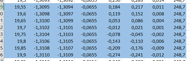
Enter the known values of initial mass, initial velocity, force of the rocket, burn rate, and desired time interval into and Excel graph. For each time interval, calculate acceleration, average acceleration, change in velocity, velocity, average velocity, change in position, and position. Fill enough rows to observe where the value of position reaches its maximum.

Data and Graphs:

Analysis:

The first photo shows the analytical approach to this problem. As evidenced by the length of equations and calculations, it is a very cumbersome method to use for this problem. The second photo shows the numerical approach to the problem where important values were calculated at each time interval to produce an approximate model of the situation. A graph was included to offer visualization of position vs time. As can be seen in the third photo, our model predicted that the maximum position reached is 248.7 meters, essentially identical to the analytically produced value of 248.7 meters.

Conclusion:

Our numerical approach was accurate enough to produce a model which predicted the desired value with adequate levels of accuracy when compared to the true value as calculated through an analytical approach. Even so, there is still uncertainty in the numerical model not found in the analytical approach. Because it is impossible to calculate infinitely small time intervals numerically, the model will, given enough iterations, begin to deviate significantly from the true value and make inaccurate predictions. For this reason, models are typically only applicable when the overall time frame of a system is small enough or the measurement scale of the system is large enough to where small inaccuracies do not severely affect the predictions. As no actual measurements were made, there was no random error present in this lab.